1Beyond three numbers of complexity

An algorithm does not have a single running cost at a fixed input size. It has a collection of possible costs, one for each input and, for randomized algorithms, each sequence of random choices. Best-case and worst-case bounds describe the extremes. Average-case analysis describes a center once a probability model has been chosen. None of these numbers, by itself, says how common the costs between the extremes are.

That missing shape can answer natural questions. Is a run moderately above average unusual? Is the long-cost side heavier than the short-cost side? If two algorithms have the same expected cost, does one vary more? Such questions call for the distribution of cost over the input and randomness space. The distribution contains the familiar summaries, but also records their arrangement: spread, asymmetry, and tails.

There are two ways to study that shape. At a given input size, one can ask which simple probability family describes the costs better. As the size grows, one can ask whether that family becomes the true limiting shape after removing the changing center and scale. A fit can win the first comparison without winning the second. Quicksort offers a clean example of this distinction.

2A distribution generated by recursive splits

We count comparisons, rather than wall-clock time, to isolate the algorithm from machine effects. Consider $n$ distinct keys. At each recursive call, choose a pivot uniformly among the keys in that subproblem, compare it with the other keys, and recurse on the two sides. Let $C_n$ be the total count. With $C_0=C_1=0$, its distribution satisfies, for $n\ge2$,

Here $\overset d=$ means equality in distribution, $I_n$ is uniform on the displayed integers, and the prime denotes an independent recursive copy. The two recursive counts are independent conditional on $I_n$. Equation (1) describes an entire distribution, not just an expected runtime. Balanced splits tend to save comparisons; repeated uneven splits increase the count.

For a small illustration, the full distribution at $n=4$ is

Its best case is $4$, worst case is $6$, and mean is $29/6$. The table says more: the middle cost is the least common of the three. For large $n$, the support and probabilities are far richer, but the same recurrence determines them.

Write $\mu_n=\mathbb EC_n$, $v_n=\operatorname{Var}(C_n)$, and $m_{r,n}=\mathbb E(C_n-\mu_n)^r$ for the mean, variance, and $r$th central moment; $\mathbb E$ and $\operatorname{Var}$ denote expectation and variance. Every $C_n$ with $n\ge2$ is strictly positive. Standard identities give [3, 2]

where $H_n^{(r)}=\sum_{j=1}^n j^{-r}$ and $H_n=H_n^{(1)}$. All logarithms below are natural unless a base is shown.

The mean grows like $n\log n$, while the standard deviation grows like $n$. Relative fluctuations shrink, even though the number of comparisons still varies substantially on the $n$ scale. This observation will matter for both results.

3Result 1: a lognormal wins the finite-size fit

A histogram of comparison counts can look somewhat bell-shaped, but with a longer right side. It is therefore natural to compare a normal density with an ordinary lognormal density; the latter is the distribution of $e^G$ for a Gaussian variable $G$. We make the phrase better fit precise: for each family, choose the parameters maximizing the expected log-density at the actual comparison count. This is a population score under the exact distribution of $C_n$, not a judgment by eye or a fit to a simulated sample.

Let $S_N(X)$ and $S_L(X)$ denote the optimal expected log-densities for normal and ordinary lognormal families when $X>0$. The normal optimum matches the mean and variance of $X$; the lognormal optimum matches the mean and variance of $\log X$ in log space. The exact score difference is

Positive $\Delta$ means that the lognormal assigns a higher expected log-density to the observed counts. Counts are discrete and these models continuous; evaluating both densities at the same count is a comparative score, not a claim that either density is the exact probability mass function.

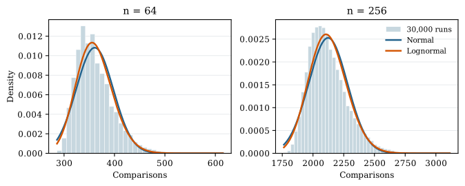
In plain terms, this comparison has no later crossover: under this particular scoring rule, the best lognormal beats the best normal at every size from four onward. The statement is stronger than a histogram comparison at a few sizes. It has a specific scope: ordinary lognormal and normal densities optimized by expected log-density. A different criterion or a shifted lognormal is a different question.

The proof turns the fit comparison into a condition on the third and fourth central moments. A useful general criterion is

Here $\min X$ is the smallest value in the support of $X$ (its essential infimum in general). The third-moment term captures rightward asymmetry; the fourth moment controls the error in approximating the logarithm. For Quicksort, exact rational interval checks establish both conditions for $4\le n<10{,}000$. Uniform analytic bounds establish them for every $n\ge10{,}000$. Appendix A provides the proof and certificate details. The calculation uses published Quicksort moment identities [3]; the all-size fit inequality is obtained by combining them with (6).

4Result 2: the fitted shape does not become exact

Winning a finite-size score comparison does not mean that Quicksort is becoming lognormal. To ask about its eventual shape, first remove the moving mean and scale:

The classical Quicksort limit theorem says that $\widehat C_n$ converges in distribution to a non-normal random variable $Q$ [1, 2]. In particular, the known moment formulas give its skewness as

Here $\operatorname{skew}(W)=\mathbb E(W-\mathbb EW)^3/(\operatorname{Var}W)^{3/2}$ for a variable $W$ with positive variance, and $\zeta(r)=\sum_{j=1}^{\infty}j^{-r}$ for $r>1$. The positive constant says that the long right side survives the passage to large inputs.

Now let $L_n$ be an ordinary lognormal with the same mean and variance as $C_n$. Its relative spread shrinks:

The $\Theta$ notation means that the ratio of the two positive quantities stays between fixed positive constants for all sufficiently large $n$. When a lognormal becomes narrow relative to its mean, its centered and standardized shape tends to a normal. Its skewness therefore tends to zero, while Quicksort’s tends to the nonzero constant above. More precisely, with $\widehat L_n=(L_n-\mu_n)/\sqrt{v_n}$,

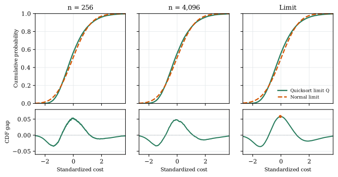
The arrow $\Rightarrow$ denotes convergence in distribution, and $\mathcal N(0,1)$ is the normal law with mean zero and variance one. The largest gap between their cumulative distribution functions (CDFs) has a positive limit:

Here $\mathcal L(Q)$ is the law of $Q$, and $d_K(A,B)$ is the supremum of the absolute difference between the CDFs of laws $A$ and $B$; it is unchanged by applying the same increasing affine transformation to both laws. This is a precise sense in which the lognormal approximation never converges to the true standardized Quicksort shape. The log-score-optimal ordinary lognormal from Result 1 also has an asymptotically normal standardized shape. Appendix B proves these statements.

5Putting the two statements together

The results describe two scales of one phenomenon. On the scale of the raw positive count, a mild right asymmetry helps a lognormal beat a symmetric normal in expected log-density. On the scale of fluctuations around the mean, random recursive splits keep an asymmetric limiting shape. A fitted lognormal becomes approximately normal on that standardized scale because its relative spread shrinks.

This distinction is useful beyond Quicksort. When an algorithm’s cost is summarized by a fitted curve, ask what the fitting rule measures and whether that curve also describes the cost after centering and scaling. A good score at every finite size and an incorrect limiting law can coexist. These results apply to the uniform-pivot comparison-count model in (1); other implementations and costs require their own analysis.

Appendix AProof of the finite-size fit result

For a positive random variable $X$, let $S_N(X)$ and $S_L(X)$ be the suprema of $\mathbb E\log f(X)$ over ordinary normal densities on $\mathbb R$ and ordinary lognormal densities on $(0,\infty)$, respectively. The normal optimizers are $\mathbb EX,\operatorname{Var}X$; the lognormal’s log-location and log-variance optimizers are $\mathbb E\log X,\operatorname{Var}(\log X)$. Direct substitution gives the exact score gap

The quantity is dimensionless: changing the unit of $X$ cancels between the two terms.

Appendix BProof of the limiting separation

The advantage above might suggest that Quicksort becomes lognormal at large $n$. Its standardized limit says otherwise. Let $L_n$ be the ordinary lognormal with the same mean $\mu_n$ and variance $v_n$ as $C_n$, and put

Appendix CExact certificate specification

This appendix records enough detail to reproduce the finite interval computation without sampling. Define $H_r=H_n^{(r)}$ and $a=n+1$. The fourth central moment used in the test is the published formula [3]

For each $n=4,\ldots,9999$, maintain four integer sums

Substitute $[S_r(n)/D,(S_r(n)+n)/D]$ for $H_r$ in (2), (15), and the expression above. Ordinary outward interval addition and multiplication produce intervals for $\mu_n,m_{3,n},m_{4,n}$. Assert that the lower endpoints of $3b_n-2\mu_n$ and $3\mu_nm_{3,n}-4m_{4,n}$ are strictly positive. The integer floor bound gives an interval containing each harmonic number, so a passing lower endpoint proves the corresponding exact inequality. The certificate reports 9,996 successful sizes; direct probability mass functions generated from (1) independently cross-check the moment formulas for $2\le n\le12$.

For the tail constants, set $M=200$ and $T_r=\sum_{j=1}^{M}j^{-r}$. Integral comparison supplies rational enclosures

They imply $1.6449<\zeta(2)<1.645$, $\zeta(3)>1.202$, and $\zeta(4)>1.0823$. Substituting these rational values into the right sides of (18) and (19), with $t=10^{-4}$, yields respectively $>0.2238$ and $<1.0194$. These estimates are deliberately looser than necessary; the displayed proof only needs $0.22$ and $1.1$. In particular, the $\log N<10$ observation controls $H_n/n$ through monotonicity of $(\log n+1)/n$; it is not applied as the false statement $\log n<10$ for all $n\ge N$.

The minimum comparison formula (14) follows from splitting as evenly as possible at every node. If $n=2^h q$ with $1\le q<2$, then $b_n/n\ge h-2/q$. Since $\log_2 q+2/q\le2$ on $[1,2]$, this implies $b_n/n\ge\log_2 n-2$. This final elementary inequality makes the analytic tail independent of the finite certificate.

References

1. U. Rösler. A limit theorem for “Quicksort.” RAIRO Theoretical Informatics and Applications, 25(1):85–100, 1991. https://www.numdam.org/item/ITA_1991__25_1_85_0/.

2. J. A. Fill and S. Janson. Quicksort asymptotics. Journal of Algorithms, 44(1):4–28, 2002. https://arxiv.org/abs/math/0105248.

3. Y. Yao. A detailed analysis of Quicksort algorithms with experimental mathematics. Manuscript, 2019. https://sites.math.rutgers.edu/~yao/QuickSort.pdf.