Frozen Deployment Under Drift

Deployment risk is a tangent-geometry problem.

Jonathan R. Landers
ORCID: 0000-0003-1872-6179

This project develops a formal account of long-horizon deployment instability for frozen predictors under dynamic covariate drift. 
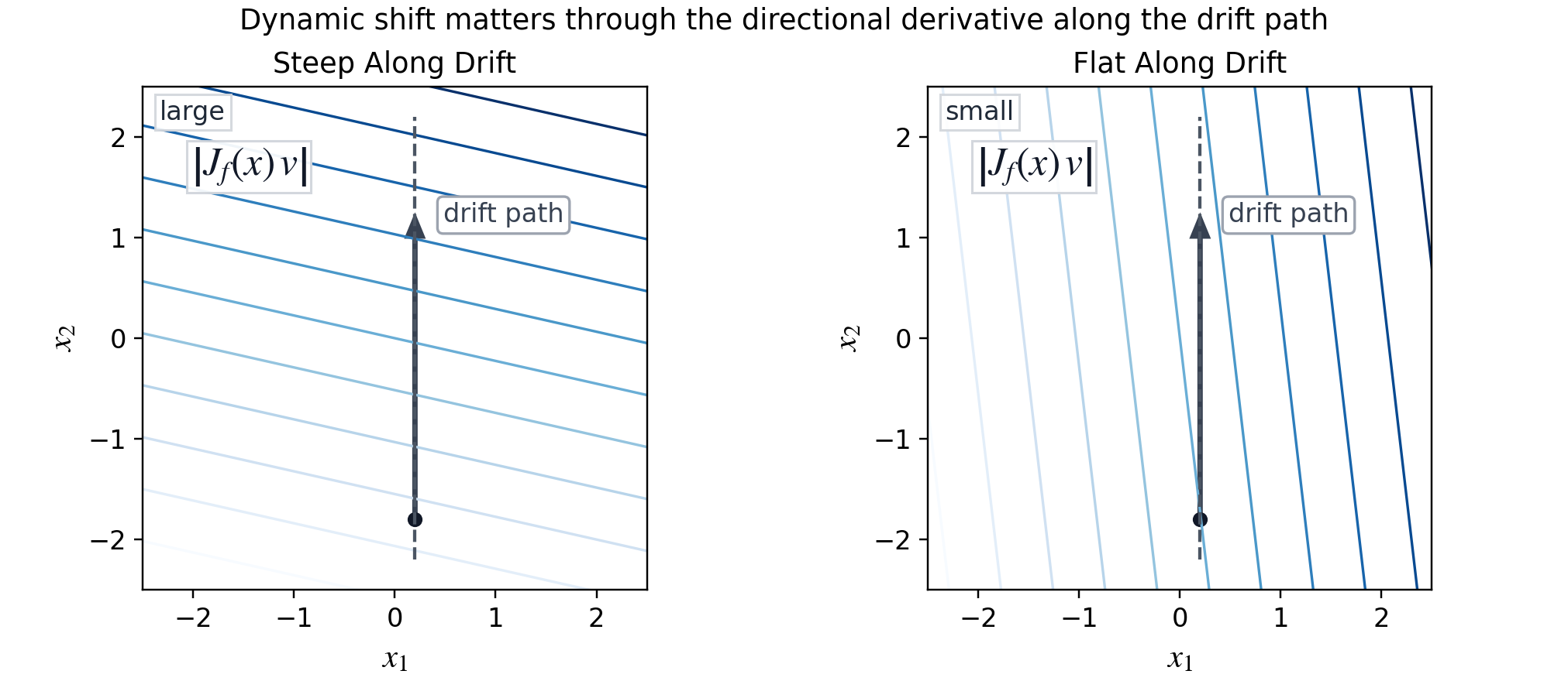
The central object is the Jacobian-velocity interaction \(J_f(X_t)\dot X_t\): environmental motion only becomes dangerous when it passes through directions where the model is locally steep.

The practical implication is that robustness should not be spread uniformly over every direction in feature space, but concentrated where deployment drift is actually expected to travel. That same directional geometry also gives a natural monitoring signal, linking training-time regularization and deployment-time volatility assessment through one coherent mechanism.

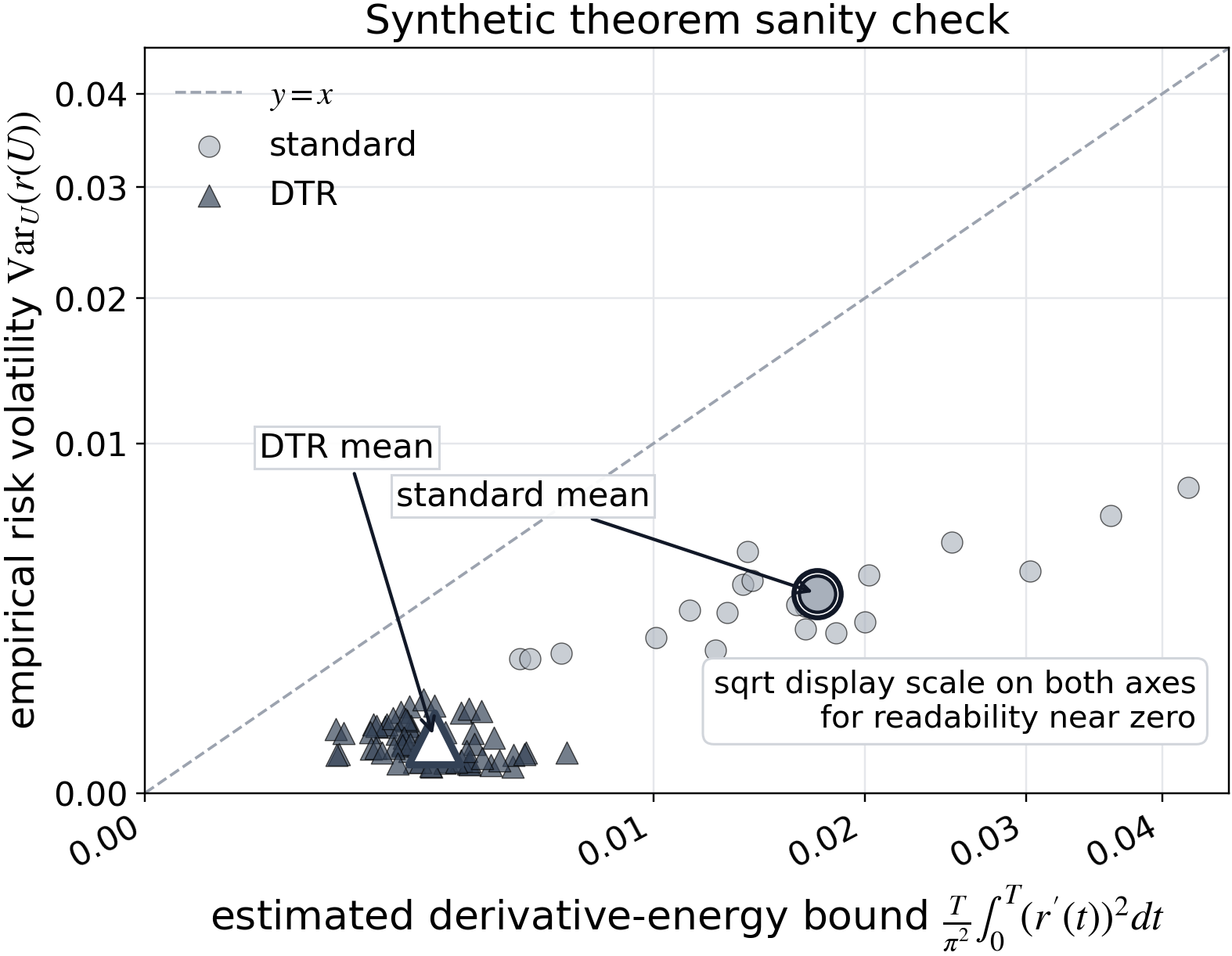
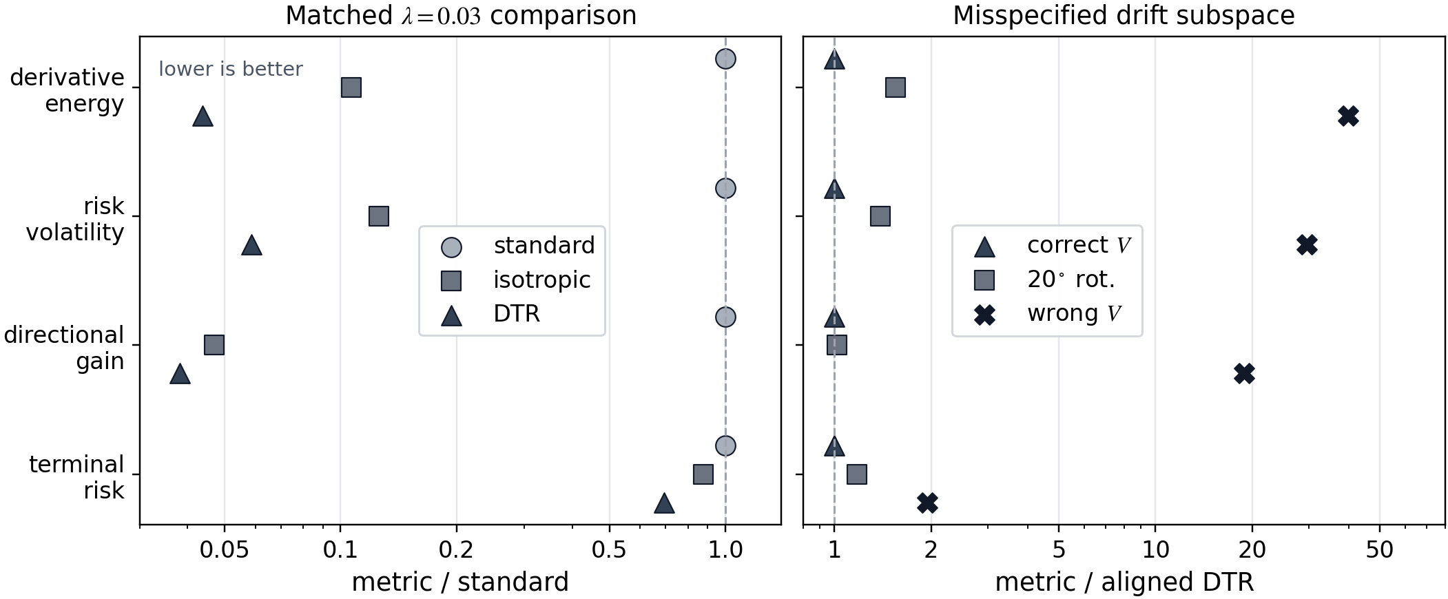
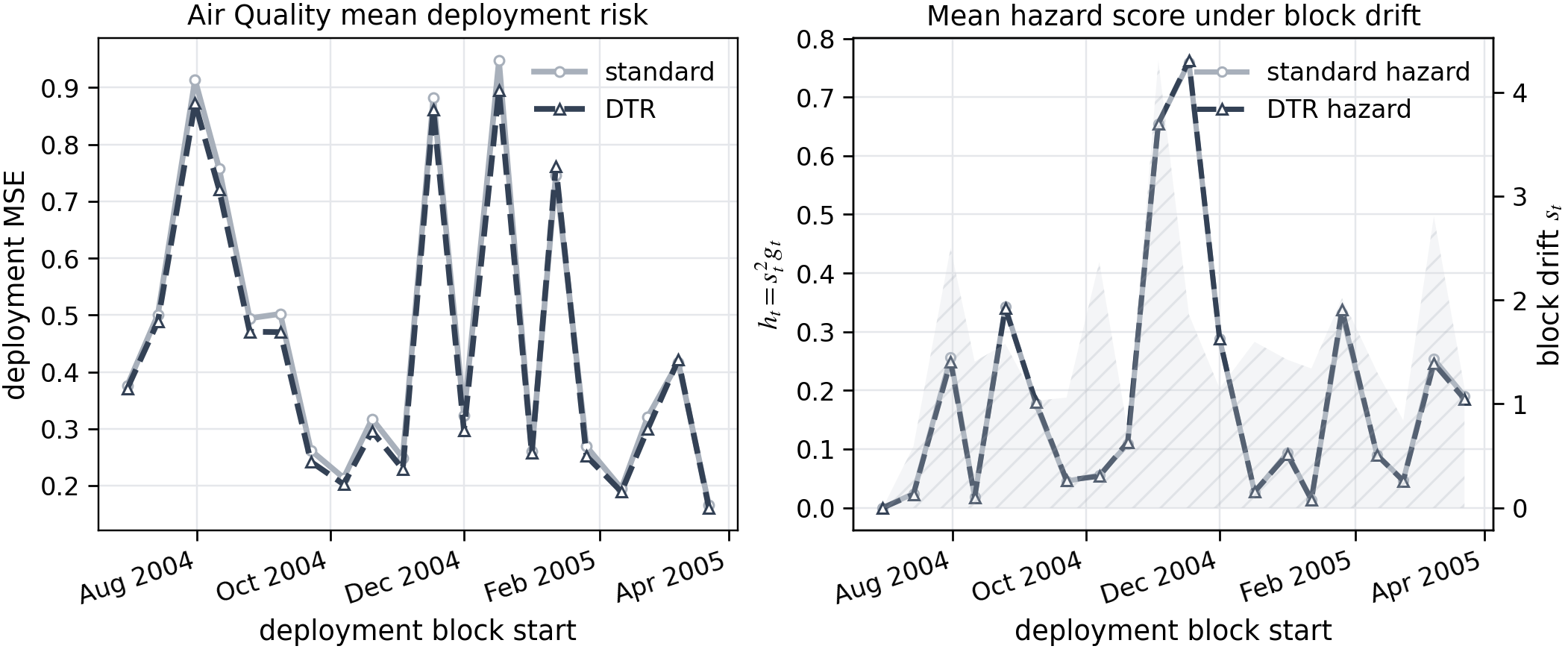
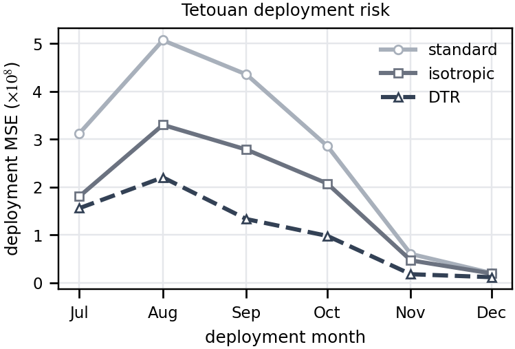
The empirical arc is deliberately staged: first verify the time-domain bound, then show that directional smoothing beats isotropic smoothing in a controlled low-rank setting, and finally test the same story on two real frozen deployments, UCI Air Quality and Tetouan City power consumption.

In the rank-1 setting, a short bookkeeping proposition makes the monitoring proxy gap explicit: block averaging, residual drift, and angular misalignment determine how the hazard proxy departs from the leading low-rank term.

The repository also includes a dedicated proof-verification suite: symbolic identities, numerical stress tests, and cached-summary checks are collected into an HTML report that follows the same visual language as this site.

92.6%Synthetic volatility reduction with DTR
9/10Air Quality DTR MSE and volatility wins vs standard
8/10Tetouan DTR volatility wins vs isotropic

Context

The paper is deliberately scoped to frozen-model deployment under continuous covariate drift: the predictor is frozen, the environment drifts continuously, and the object of interest is a deployment-risk trajectory rather than a single train-test shift gap.

The setup

\[ r(t):=\mathbb{E}[g_\theta(X_t)]. \]

The model \(f_\theta\) stays fixed after training while covariates evolve as \(X_t\). Instability is therefore temporal and geometric.

  • Frozen predictor \(f_\theta : \mathbb{R}^d \to \mathbb{R}\)
  • Dynamic covariate path \(X_t\)
  • Risk volatility measured over \(t \in [0,T]\)

The mechanism

\[ J_f(X_t)\dot X_t \]

The same drift path can be benign for one model and harmful for another. What matters is whether motion aligns with locally steep predictor directions.

  • Flat tangent directions make drift comparatively mild
  • Steep tangent directions turn motion into volatility
  • The theorem isolates this interaction explicitly

The payoff

\[ \begin{gather*} \mathcal{L}_{\mathrm{DTR}}(\theta) = \\ \mathbb{E}\ell(f_\theta(X),Y) + \lambda \mathbb{E}\|J_f(X)V\|_F^2 \end{gather*} \]

Once the drift geometry is estimated, robustness should be enforced in those directions instead of spread uniformly across the ambient space.

  • Directional regularization instead of isotropic Jacobian smoothing
  • Monitoring score aligned with the same geometry
  • One theorem-to-method story from synthetic to field deployment

Main Mathematical Results

The formal story is compact: control temporal volatility by derivative energy, control derivative energy by Jacobian-velocity energy, then specialize to low-rank drift. A short bookkeeping proposition quantifies the rank-1 monitoring proxy gap.

Lemma 1

\[ \begin{gather*} \mathrm{Var}_U(r(U)) \le \\ \frac{T}{\pi^2}\int_0^T (r'(t))^2dt. \end{gather*} \]

Large volatility requires large derivative energy somewhere along deployment time.

Theorem 1

\[ \begin{gather*} \mathrm{Var}_U(r(U)) \le \\ \frac{\beta^2 T}{\pi^2}\int_0^T \mathbb{E}\!\left[\|J_f(X_t)\dot X_t\|^2\right]dt. \end{gather*} \]

Deployment instability is driven by accumulated tangent amplification of realized motion.

Corollary 1

\[ \begin{gather*} \dot X_t = Va_t+\rho_t, \\ V^\top V = I_k. \end{gather*} \]

In low-rank regimes, the leading term is directional Jacobian energy in the drift subspace.

Proposition 1

\[ \begin{aligned} s_t^2 &= |\bar a_t|^2 + \|\bar\rho_t\|^2, \\ g_t &= \cos^2\theta_t\,G_{\parallel,t} + \sin^2\theta_t\,G_{\perp,t} + 2\sin\theta_t\cos\theta_t\,C_t. \end{aligned} \]

In the rank-1 monitoring setting, block averaging contributes residual drift energy, while angular misalignment mixes aligned, orthogonal, and overlap energies. This bookkeeping result explains how the monitoring proxy departs from the leading low-rank term.

A1Deployment paths are absolutely continuous with finite velocity energy.
A2The performance field admits a valid chain rule along the trajectory.
A3Directional changes in the performance field are dominated by score-Jacobian changes along deployment.
Operational viewFlatten the predictor where future motion is likely, then monitor the same directional mechanism during deployment.

Proof Verification

The mathematical claims are paired with an explicit verification layer: exact symbolic checks for the theorem chain and hazard-score bookkeeping, numerical stress tests for the low-rank inequalities, and consistency checks against the cached synthetic summaries used by the plotting code.

Exact Identities

\[ \mathrm{Var}_U(r(U)) \le \frac{T}{\pi^2}\int_0^T (r'(t))^2dt \]

SymPy checks the core algebra exactly rather than numerically: the Poincaré sharpness example, a deterministic equality case for the Jacobian-velocity theorem, the composition-chain identity behind A3, the rank-1 hazard-score bookkeeping identity, and the Bernoulli cross-entropy derivative bound.

  • Equality case for the temporal bound
  • Exact chain-rule factorization in the composition setting
  • Pointwise rank-1 bookkeeping underlying the monitoring proposition
  • Closed-form derivative bound for soft-target cross-entropy

Numerical Stress Tests

\[ \begin{aligned} \|M(Va+\rho)\|^2 &\le 2\|MV\|_F^2\|a\|^2 \\ &\quad + 2\|M\rho\|^2 \end{aligned} \]

Some parts of the argument are more naturally checked by dense quadrature or randomized linear-algebra trials. The verification suite therefore stress-tests the low-rank corollary and a smooth expectation-based example of the full theorem chain.

  • Randomized orthonormal-basis checks for the corollary inequalities
  • Smooth expectation example verifying \(\mathrm{Var} \le\) chain bound \(\le\) Jacobian-velocity bound
  • Tolerance-aware validation for cached numerical summaries

Styled HTML Report

python proof_verification/generate_report.py

Running the verifier writes a machine-readable JSON summary and an HTML report that reuses this site's fonts, palette, card layout, and MathJax setup.

Experimental Results

The experiments mirror the theorem-to-method pipeline: visualize the geometry, verify the time-domain step in a clean synthetic benchmark, compare directional and isotropic smoothing, then test the same story on two real frozen deployments.

Geometry figure comparing steep versus flat tangent directions along the same drift path.
Figure 1

Geometric intuition

The deployment path is identical in both panels. Only tangent geometry changes. Drift is dangerous only when it aligns with steep local directions of the predictor.

  • Conceptual quantity\(J_f(x)v\)
  • TakeawayDrift magnitude alone is not enough
  • Design implicationRegularize along drift directions
Synthetic time-domain sanity check figure.
Figure 2

Synthetic time-domain sanity check

Each point is one trained model evaluated over the drifting synthetic path. DTR moves the cloud toward lower derivative energy and lower volatility.

  • Standard volatility\(3.25\times10^{-3}\)
  • DTR volatility\(2.39\times10^{-4}\)
  • Volatility reduction92.6%
  • Directional-gain reduction95.5%
Directional ablation comparing DTR, isotropic smoothing, and misspecified drift subspaces.
Figure 3

Directional beats isotropic

At matched \(\lambda=0.03\), DTR improves on both the standard model and isotropic Jacobian regularization across derivative energy, volatility, directional gain, and terminal risk.

  • Standard terminal risk0.189
  • Isotropic terminal risk0.165
  • DTR terminal risk0.131
  • Wrong-subspace volatility inflation29.6x
Air Quality deployment figure showing blockwise MSE and hazard score.
Figure 4

Field deployment on UCI Air Quality

The real-data study freezes the regressor, estimates a target-orthogonal sensor-drift subspace from unlabeled deployment covariates, and evaluates blockwise MSE over 20 biweekly deployment blocks. With that more focused nuisance-drift subspace, validation-selected DTR improves deployment MSE and volatility against standard training.

  • Standard volatility\(0.073\pm0.023\)
  • Validation-selected DTR volatility\(0.069\pm0.020\)
  • DTR MSE wins vs standard9/10 seeds
  • DTR volatility wins vs standard9/10 seeds
  • Roll-2 monitor vs next \(\Delta r^2\)0.307
  • All-covariate subspace checkover-regularizes
Tetouan deployment figure showing monthly blockwise MSE for standard, isotropic, and DTR models.
Figure 5

Second real benchmark: Tetouan power

The paper adds a second real frozen-deployment study on the UCI Tetouan City power-consumption dataset, predicting Zone 1 load from weather and diffuse-flow covariates across six monthly deployment blocks in late 2017. Validation-selected DTR gives the strongest real-data stability result.

  • Deploy MSE, standard / isotropic / DTR1.08e8 / 1.01e8 / 6.82e7
  • Volatility, standard / isotropic / DTR1.07e16 / 7.20e15 / 3.07e15
  • DTR volatility wins vs standard8/10 seeds
  • DTR volatility wins vs isotropic8/10 seeds
  • Roll-2 monitor vs next \(\Delta r^2\)0.305

Repository

The repo is organized to be readable both as a paper companion and as a reproducible verification package: manuscript, cached summaries, figures, proof checks, and training scripts are all included.

What lives where

  • ManuscriptPDF and LaTeX source for the paper.
  • scripts/Training, evaluation, reporting, and plotting code for the synthetic theorem benchmark, directional ablation, Air Quality study and subspace ablation, Tetouan figure, real-data paired comparisons, and monitoring-volatility ablation.
  • benchmark_package/Isolated Tetouan benchmark package used for the paper's second real deployment study, with cached matched-seed outputs, a dedicated runner, and benchmark-selection notes.
  • proof_verification/SymPy-based checks, numerical stress tests, and the generated HTML/JSON verification reports.
  • figures/Rendered manuscript figure assets, now including the Tetouan deployment plot, plus cached CSV/JSON summaries consumed by the plotting scripts.
  • data/Cached Air Quality dataset used by the main field-deployment experiment.

Quick Start

Install the Python dependencies, regenerate the manuscript figure assets and real-data reports, run the verification suite, and use the isolated Tetouan benchmark package to reproduce the paper's second real deployment study.

python -m venv .venv
.venv\Scripts\Activate.ps1
pip install -r requirements.txt
python scripts/generate_all_figures.py --force
python scripts/run_real_deployment_reporting.py --force
python proof_verification/generate_report.py
python benchmark_package/scripts/run_tetouan_power_benchmark.py --force
latexmk -pdf jacobian_velocity_bounds_deployment_risk_covariate_drift.tex